Summary of Day 51:

*Starting of Chapter 16- Deep Learning

Intro basics:

Core Equation:
Most machine learning tasks use:
\(y = Wx + b\)

• $W$: Weight matrix
• $x$: Input
• $b$: Bias

Classifier Function:
A model \(f(x; \theta)\) maps inputs to labels:

• $\theta = (W, b)$: Parameters learned from data

Perceptron (Linear Classifier):
\(y = \text{sign}(Wx + b)\)

• Sign activation: Outputs ${-1, 0, 1}$ based on input sign
• Introduces nonlinearity for classification

Decision Boundary:

• Linear equation $Wx + b = 0$ splits input space into regions
• Example (2D): $w_1x_1 + w_2x_2 + b = 0$ defines a line

Inference:
Compute class labels by evaluating $\text{sign}(Wx + b)$.

ⓘ Note: This is just a revision note. Assuming readers have prior knowledge of these topics.

Multilayer Classifiers:

Okay, so Linear Classifiers use hyperplanes (lines in 2D, planes in 3D) to partition the input space into regions, each representing a class.

However, the major limitation is that not all datasets can be separated by a single hyperplane. For example:

Let’s take this image graph:

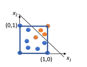
Fig 51_01: Single Layer Perceptron

Here, in the above image, the classifier failed to properly classify that single “orange” point.

So that’s where Multilayer Perceptrons (MLPs) come in.

• MLPs overcome this limitation by using multiple layers of perceptrons
• Each layer transforms the input space into a new feature space, enabling more complex classification patterns.

Example: Two Layer Perceptron:

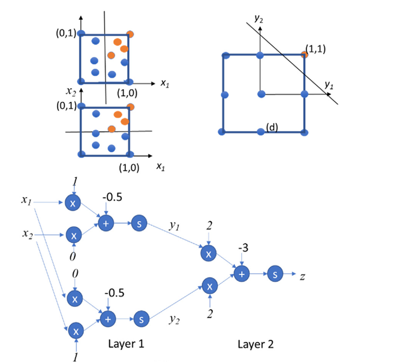
Fig 51_02: Two Layers Perceptron

So here:

Layer $1$: Transforming Input Space

• Layer $1$ consists of two perceptrons.
  • $y_1 = \text{sign}(x_1 - 0.5)$ : Classifies points based on $x_1 > 0.5$.
  • $y_2 = \text{sign}(x_2 - 0.5)$ : Classifies points based on $x_2 > 0.5$.
• Outputs of Layer $1$ $(y_1 , y_2)$ are restricted to nine possible combinations: $(−1,−1),(−1,0),(−1,1),(0,−1),(0,0),(0,1),(1,−1),(1,0),(1,1)$

Layer $2$: Final Classification

• Layer $2$ uses a single perceptron to classify points in the transformed $y_1 - y_2$ space:
  • A line like $z= \text{sign}(2y_1 + 2y_2 -3)$ seperates the orange points $((y_1, y_2)= (1,1))$ from others.

Need for More Layers:

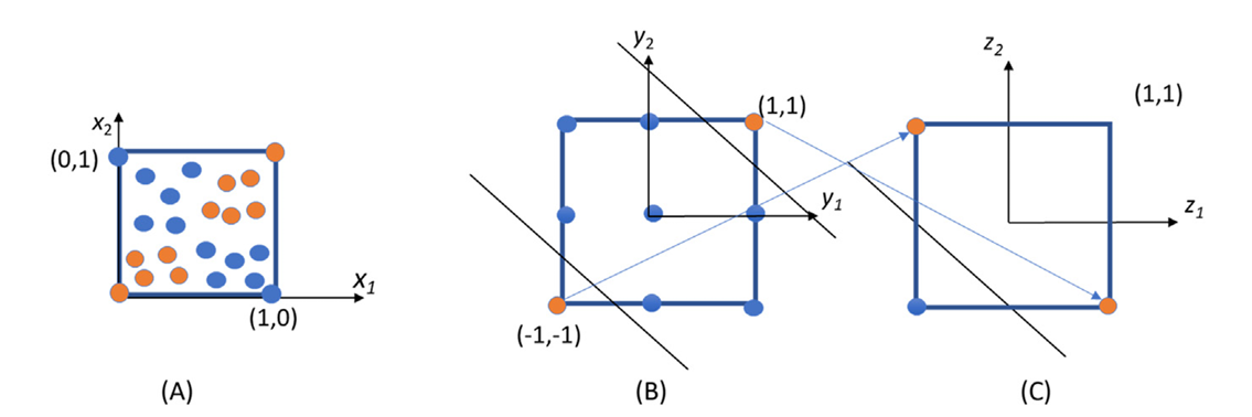
Fig 51_03: Need for perceptrons with more than two layers

Problem with Two Layers:

A two-layer perceptron cannot classify datasets like the one in Figure 51_03(A), where orange points form two disjoint regions.

Solution: Adding Another Layer

• Adding a third layer enables proper classification:
  • Layer 2 introduces additional transformations $(z_1, z_2)$ in the second feature space.
  • A line like $z_1 + z_2 + 1 = 0$ seperates the classes in final feature space $(z_1 - z_2)$.

ⓘ Disclaimer: In book there are different terminologies which assuming every one knows, not including here. Topics excluded:

• Error Function
• SGD
• Epoch
• BackProp
• Chain Rule
• Learning Rate
• Minibatch: Splitting the training data into smaller subsets or batches during the training process
• Feed Forward Network

---

Now let’s dive towards the real deep learning stuffs…

CNNs (Convolutional Neural Networks):

Well, we did study about convolutions in Chapter 7 earlier. Now let’s bridge this to deep learning.

---

Core Components of CNNs

1. Convolutional Layers:
   • Purpose: Extract hierarchical features (edges → textures → complex patterns).
   • Mechanism: Apply filters (kernels) to local input regions.
     • Example: A $3×3$ filter scans the input, computing dot products.
   • Key Concepts:
     • Weight Sharing: Same filter used across all input patches → reduces parameters.
     • Feature Maps: Outputs highlight detected features.
2. Subsampling (Pooling) Layers:
   • Purpose: Reduce spatial size, retain critical features.
   • Types:
     • Max-Pooling: Takes maximum value in a patch (e.g., $2×2$).
     • Average-Pooling: Takes average value in a patch.
3. Fully Connected Layers:
   • Role: Combine high-level features for classification.
   • Math:
     \(Y = W \cdot X + b\)
     • $W$: Weight matrix, $X$: Input, $b$: Bias.

---

LeNet-5 Architecture

• Structure:
  

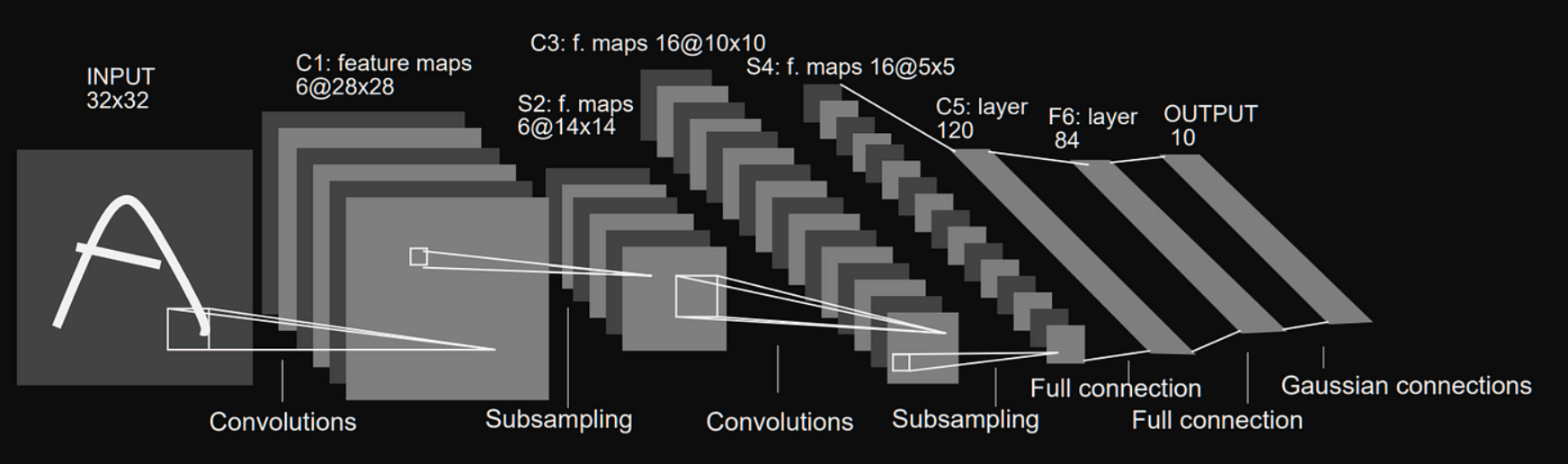
  Fig 51_04: LeNet-5 Architecture

  1. Input: $32×32$ grayscale image (handwritten digit).
  2. Conv Layers: Extract spatial features (edges, curves).
  3. Subsampling: Reduce dimensionality (focus on essential patterns).
  4. Fully Connected Layers: Output probabilities for $10$ digit classes.

---

Training CNNs

1. Supervised Learning:
   • Input: Labeled data (e.g., images tagged with digits).
   • Error Function:
     \(E = \frac{(y - t)^2}{2}\)
     • $y$: Predicted output, $t$: True label.
2. Stochastic Gradient Descent (SGD):
   • Update Rule:
     \(w_i = w_i - \epsilon \frac{\partial E}{\partial w_i}\)
     • $\epsilon$: Learning rate.
3. Backpropagation:
   • Computes gradients via chain rule:
     \(\frac{\partial E}{\partial w_i} = \frac{\partial E}{\partial y} \cdot \frac{\partial y}{\partial w_i}\)
   • Propagates errors backward to adjust weights.

---

Why CNNs Work

• Hierarchy: Automatically learns low → high-level features.
• Efficiency:
  • Parameter Sharing: Fewer parameters than fully connected networks.
  • Spatial Invariance: Detects patterns regardless of position.

---

Okay, enough of theory, let’s code as well. This time first write some code based on C (not going into kernels and parallization yet!)

Click Here to redirect to the code implementation.