Summary of Day 61:

So, today I fixed yesterday’s MHA triton implementation. Took a lot of time so not going into CUDA today. However, will explain the code mechanism in very minute detail so that everyone could understand. Also, this would be a revision for me.

Understanding the $Q, K, V$ kernel:

Firsty, let’s understand the parameters defined in this kernel.

def qkv_kernel(
    input_ptr, 
    wq_ptr, wk_ptr, wv_ptr, 
    bq_ptr, bk_ptr, bv_ptr, 
    q_ptr, k_ptr, v_ptr,
    batch_size: tl.constexpr, seq_len: tl.constexpr, embed_dim: tl.constexpr,
    head_dim: tl.constexpr, num_heads: tl.constexpr, stride_batch: tl.constexpr,
    stride_seq: tl.constexpr, stride_head: tl.constexpr
):

So, here:

• input_ptr: Pointer to the input tensor; shape of [batch_size, seq_len, embed_dim].
• wq_ptr, wk_ptr, wv_ptr : Pointer to the weights matrics for query, weight and vector. Shape of [num_heads * head_dim, embed_dim].
• bq_ptr, bk_ptr, bv_ptr : Pointer to the bias matrics for query, weight and vector. Shape of [num_heads * head_dim].
• q_ptr, k_ptr, v_ptr: Pointers to the output tensors. Shape of [batch_size, num_heads, seq_len, head_dim].
• batch_size: Number of samples in a batch. Defines how many independent inputs are processed in parallel. Used to ensure the batch_idx does not exceed valid range.
• seq_len: Length of the sequence (number of tokens). Specifies how many positions in the sequence need $Q, K, V$ projections.
• embed_dim: Dimension of input embeddings
• head_dim: Dimensionality of each attention heads (embed_dim // num_heads)
• num_heads: Number of attention heads in MHA
• stride_batch: The memory stride between consequtive batches. Multiplied with batch_idx to compute the base offset of a batch
• stride_seq: The memory stride between consequtive sequences. Multiplied with seq_idx to compute offset for a specific position.
• stride_head: The memory stride between consequtive heads. Multiplied with head_idx to access the data for a specific head.

Now explaining the inner mechanism:

• First comes thread indexing and bounds checking. The kernel is launched with a 3D grid size of (batch_size, seq_len, num_heads).

• Next, memory offset calculation:
  • The input_offset is quite simple. It points to the start of the input vector for the current batch and sequence position.
  • In qkv_offset, we even account for the heads, hence adding the heads offset. (as $Q, K, V$ are split across heads)
• Now comes projection loop:
  • The outer loop: (d loop)
    • Iterates over the output dimension (head_dim), computing one element of $Q, K \text{ and } V$. Since each element needs a full dot product.
  • The inner loop: (e loop)
    • Iterates over the input dimension (embed_dim), performing the dot product.

[!Note] Does the dot product by multiplying and summing accross the input vector and one row of the weight matrix.

[!important] How this whole thing works:

• The Outer loop’s setup:
  • acc_q, acc_k, acc_v are accumulators (like temporary variables) initialized with bias values.
  • Bias is fetched from memory: bq_ptr + head_idx * head_dim + d picks the bias for this head and this output element.
  • Think of d as the “index” of the output vector we’re filling.
• The Inner Loop:
  • Loads one input element: x_val = tl.load(input_ptr + input_offset + e).
  • Loads one weight from each matrix:
    • wq_val from $WQ$ at row (head_idx * head_dim + d), column e.
    • wk_val from $WK$, same row and column.
    • wv_val from $WV$, same row and column.
  • Multiplies and adds to accumulators:
    • acc_q += x_val * wq_val (Query dot product).
    • acc_k += x_val * wk_val (Key dot product).
    • acc_v += x_val * wv_val (Value dot product).

[!note] For one output element (d), we multiply the entire input vector by one row of the weight matrix and sum the results.

The attention_kernel:

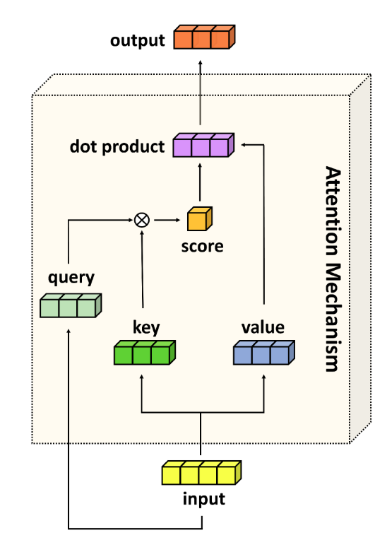
Fig 61_01: Attention Mechanism

Params recap:

• Pointers: q_ptr, k_ptr, v_ptr (inputs), scores_ptr (intermediate scores), output_ptr (final output).
• Dimensions: batch_size, seq_len, head_dim, num_heads define the tensor shapes.
• Strides: stride_batch, stride_seq, stride_head navigate memory.
• Scale: scale = 1/sqrt(head_dim) normalizes the dot product.

Thread initalization and boundary check:

• similar to above.

Memory Offsets:

• q_offset = batch_idx * stride_batch + seq_idx * stride_seq + head_idx * stride_head
  • Points to the start of the Query $(Q)$ vector for this thread’s (batch_idx, seq_idx, head_idx) in the $Q$ tensor.
  • Shape of $Q$: [batch_size, seq_len, num_heads, head_dim]- $4D \text{ tensor.}$
• scores_offset = batch_idx * seq_len * num_heads * seq_len + seq_idx * num_heads * seq_len + head_idx * seq_len
  • Shape of scores: [batch_size, seq_len, num_heads, seq_len]

[!important]

• The batch_idx * seq_len * num_heads * seq_len shifts the offset for the batch. Here we account for all the attention socres in previous batches, each of which has seq_len * num_heads * seq_len scores.
• seq_idx * num_heads * seq_len moves to the correct query position in the sequence. Each query position has num_heads * seq_len scores (because each head generates a score for each key position).
• head_idx * seq_len moves to the correct attention head for a given query.

[!Caution] The order of multiplication matters!!

Explaining this with an example:

• seq_len * num_heads * seq_len: This keeps the memory layout in a format that:
  • first: traverses all sequence lengths (for queries),
  • then iterates over all heads,
  • and finally over the keys.

This is how it’s structured to take advantage of memory access patterns when we’re iterating over the tensor.

• If we change this to num_heads * seq_len * seq_len:
  • This would change the memory access pattern. With this order, you’d:
    • First iterate over heads,
    • then over query positions,
    • and lastly over key positions.

This could work too, but it would lead to a different way of accessing memory, which might not be as efficient in certain cases, especially in terms of how the data is loaded into cache.

[!tip]

• Use seq_len * num_heads * seq_len for storing attention scores!

✅ Why?

• Keeps all values for a single query together → faster softmax & attention
• Better GPU memory coalescing → fewer trips, less latency

• Avoids cache misses → speeds up computation

• ❌ Avoid num_heads * seq_len * seq_len → Scatters data, slows down memory access!

• Rule of Thumb: Always structure memory for contiguous access!

Computing Attention Scores:

\[\text{Attention}(Q, K, V) = \text{softmax}\left(\frac{QK^T}{\sqrt{d}}\right)V\]

• So, next we calulate the Q * K^T:
  • Here we have not explicitly used any transpose operation. Instead, we are defining the offset values of $Q$ and $K$ such that there is no need to physically transpose $K$.

[!important] The q_offset is calculated as:

q_offset = batch_idx * stride_batch + seq_idx * stride_seq + head_idx * stride_head

This means for each query, we’re accessing the query vector for a specific batch, sequence position and batch index.

The k_offset changes slightly:

k_offset = batch_idx * stride_batch + k_seq * stride_seq + head_idx * stride_head

The crucial change here is that instead of using seq_idx (the query sequence index) as in q_offset, we’re using k_seq (the loop variable) to access the key vector at each position in the sequence. This allows us to access all of the keys for a given query sequence position.

Why this works:

• By modifying the offset for $K$, we allow the query vector at a given position to “align” with each key vector from the sequence (looping through k_seq).
• This results in a dot product that’s essentially the same as multiplying $Q$ with $K^T$.

Softmax Calculation:

Next, we have softmax calculation:

\[\text{Softmax}(X_i) = \frac{e^{x_i}}{\sum_{j=1}^{n} e^{x_j}}\]

• First we find the max score for numerical stability.
  • We initialize the max_score to negative infinity.
  • Then we iterate over all sequence positions (k_seq), loading the score values.

• Numerical instability could be caused by large exponentiated values.

• Then, the sum calculation part:
  • We subtract max_score from each score before exponentiating (to prevent the overflow).
  • Then we store the exponentiated values in scores_base.
  • And then we accumulate.
• Next we divide; hence getting the activation function.

---

And that’s how the kernel works.

[!Note] Explaining the wrapper function

• We start with scale = 1.0 / math.sqrt(head_dim) to normalize attention scores later. Since head_dim is embed_dim // num_heads, we take the square root to scale down dot products in Q * K^T, preventing them from growing too large and destabilizing the softmax in the attention_kernel. For example, if head_dim=4, scale=0.5.
• Next, we grab weights and biases from attention_layer (a PyTorch MultiheadAttention object). Its in_proj_weight is a big tensor [3*embed_dim, embed_dim]—three stacked weight matrices for Query (Q), Key (K), and Value (V).
• We slice wq = attention_layer.in_proj_weight[:embed_dim].T to get the Query weights, the first embed_dim rows. We transpose it (.T) from [embed_dim, embed_dim] to [embed_dim, embed_dim] because Triton kernels expect weights in [out_dim, in_dim] format, unlike PyTorch’s default. This projects input to Q.
• We do the same for wk = attention_layer.in_proj_weight[embed_dim:2*embed_dim].T (Key weights) and wv = attention_layer.in_proj_weight[2*embed_dim:].T (Value weights), slicing the next chunks and transposing them. Each is [embed_dim, embed_dim], tailored for K and V projections.
• For biases, we check in_proj_bias (size 3*embed_dim or None). If it exists, we slice bq = attention_layer.in_proj_bias[:embed_dim] for Query, bk = attention_layer.in_proj_bias[embed_dim:2*embed_dim] for Key, and bv = attention_layer.in_proj_bias[2*embed_dim:] for Value—each embed_dim-sized. If None, we use torch.zeros(embed_dim, device=DEVICE) to create zero tensors on the GPU (CUDA), ensuring no bias offset when the layer skips it.
• We grab wo = attention_layer.out_proj.weight ([embed_dim, embed_dim]) and bo = attention_layer.out_proj.bias ([embed_dim] or None, defaulting to torch.zeros) for the final output projection. No transpose here—PyTorch’s linear expects [out_dim, in_dim], which matches wo.
• We allocate output tensors on the GPU with torch.empty: q, k, v as [batch_size, seq_len, num_heads, head_dim] for Q, K, V projections. These are initially uninitialized (faster than zeros) since qkv_kernel fills them.
• We set scores = torch.zeros(batch_size, seq_len, num_heads, seq_len, device=DEVICE, dtype=torch.float32) as a 4D tensor for attention scores. We use zeros to initialize it cleanly—attention_kernel overwrites it with raw scores, then softmax weights.
• We also allocate output = torch.empty(batch_size, seq_len, num_heads, head_dim, device=DEVICE) for the attention result, uninitialized since attention_kernel populates it.
• We define a 3D grid grid_qkv = (batch_size, seq_len, num_heads) and launch qkv_kernel with it. This grid means one thread per (batch, seq, head) combo—e.g., for [2, 8, 4], that’s 64 threads. We pass input_tensor, weights (wq, wk, wv), biases (bq, bk, bv), output tensors (q, k, v), and shape/strides. It computes Q, K, V in parallel.
• We reuse the same grid grid_attn = (batch_size, seq_len, num_heads) for attention_kernel. We pass q, k, v, scores, output, shape/strides, and scale. This computes attention: softmax(Q * K^T * scale) * V, filling output.
• We reshape output from [batch_size, seq_len, num_heads, head_dim] to [batch_size * seq_len, embed_dim] (e.g., [2, 8, 4, 4] → [16, 16]) by flattening the head dimension. This concatenates head outputs, mimicking transformer behavior.
• We apply torch.nn.functional.linear(output, wo, bo)—a matrix multiplication with wo and bias addition with bo—to project the concatenated result back to embed_dim. This gives us [batch_size * seq_len, embed_dim].
• We reshape again to [batch_size, seq_len, embed_dim] (e.g., [2, 8, 16]) to match the input shape, making it usable in a PyTorch pipeline.
• Finally, we return this tensor—the multi-head attention output, ready for downstream layers.