Summary of Day 31:

Detailed Explanation of Kogge Stone Algo Continued

Okay, So today let’s dive deeper into this Algo and try to understand its mechanism, why we are using this and code implementation in more detailed way.

1. So what is Kogge-Stone Algo?

Answer: The Kogge-Stone algorithm is a parallel prefix sum algorithm optimized for fast execution with minimal dependencies.

2. Slight Overview:

The algo operates on an array $\text{XY}$ that initially contains the input elements.
It iteratively evolves the contents of $\text{XY}$ into cumulative sums (inclusive/exclusive scan) by leveraging a binary tree structure.
After $\text{log}_{2}(N)$ iterations, where $N$ is the number of elements in the array, all cumulative sums are finalized.

3. Inclusive Prefix Sum Algorithm

Algorithm Steps

Initialization

The input array $\text{X}$ is loaded into $\text{XY}$.
Each element $\text{XY}[i]$ initially contains $\text{X}[i]$.

Iterations

for $k = 0$ to $\log_2(N) - 1$:

Compute the stride as $2^k$.
For each element $i$:
```
  XY[i] = XY[i] + XY[i - \text{stride}]
```
- Otherwise, leave $XY[i]$ unchanged.

Final State

After all iterations, $\text{XY}$ contains the inclusive scan results.

Example with a $16$- Element Array

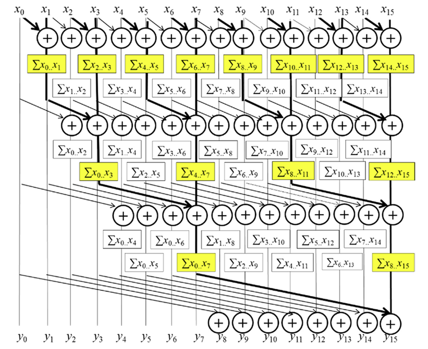
Fig 31_01: A parallel inclusive scan algorithm based on Kogge-Stone adder design.

Step-by-step Execution:

Initial State: Each element in $\text{XY}$ contains its corresponding input value:
```
\text{XY} = [x_0, x_1, x_2, ..., x_{15}]
```
Iteration 1 (Stride= 1): Each element $XY[i]$ is updated by adding it’s immediate left neighbour $(XY[i-1])$
```
\text{XY} = [x_0, x_0 + x_1, x_1+x_2, ..., x_{14}+x_{15}]
```
Iteration 2 (Stride= 2): Each element $XY[i]$ is updated by adding the value two positions into its left $(XY[i-2])$:
```
\text{XY}= [x_0, x_0 + x_1, x_0+x_1+x_2, x_0+x_1+x_2+x_3, ... ]
```
Iteration 3 (Stride= 4): Each element $XY[i]$ is updated by adding the value four positions into its left $(XY[i-4])$:

\text{XY}= [x_0, x_0 + x_1, x_0+x_1+x_2, x_0+x_1+x_2+x_3, x_0+x_1+x_2+x_3+x_4, ... ]

Continue untill all cumulative sums are computed.

After $\log_2(16) = 4$ iterations, the final array contains all cumulative sums.

Implementation:

Click Here to redirect towards complete inclusive scan.

Click Here to redirect towards complete exclusive scan.

So how different is Exclusive from Inclusive?

Answer:

The main difference between inclusive and exclusive prefix sums lies in whether the current element is included in the sum.

Inclusive Prefix Sum:

Each element in the output array is the sum of all elements up to and including the corresponding element in the input array.
In other words, the $i$-th element of the output array is the sum of the first $i$ elements of the input array.
The last element of the output array is the sum of all elements in the input array.

Exclusive Prefix Sum:

Each element in the output array is the sum of all elements before the corresponding element in the input array.
In other words, the $i$-th element of the output array is the sum of the first $i-1$ elements of the input array.
The first element of the output array is always zero.
The last element of the output array is the sum of all elements except the last one in the input array.

Example

Let’s consider an input array:

Input: [1, 2, 3, 4, 5]

Inclusive Prefix Sum:

Output: [1, 3, 6, 10, 15]

Exclusive Prefix Sum:

Output: [0, 1, 3, 6, 10]

Implementation Difference

The exclusive scan can be implemented by performing an inclusive scan and then shifting the array to the right by one position and setting the first element to zero.

Fig 31_02: A parallel exclusive scan algorithm based on Kogge-Stone adder design.

Algorithm Steps for Exclusive Scan

Initialization:

The input array $X$ is loaded into $XY$.
Each element $XY[i]$ initially contains $X[i]$.

Iterations:

for $k = 0$ to $\log_2(N) - 1$:
- Compute the stride as $2^k$.
- For each element $i$:
  - If $i \geq \text{stride}$, update:
```
XY[i] = XY[i] + XY[i - \text{stride}]
```
  - Otherwise, leave $XY[i]$ unchanged.

Shift Right:

Shift all elements in $XY$ one position to the right.
Set $XY[0]$ to 0.

Final State:

After shifting, $XY$ contains the exclusive scan results.

Complexity Analysis of Kogge-Stone Algorithm

Time Complexity

Number of Iterations: The algorithm performs $\log_2(N)$ iterations.
Work per Iteration: In each iteration, each element (or at least half of the elements) potentially performs one addition. In parallel this happens in constant time.
Overall: Since we have $\log_2(N)$ iterations and each iteration takes constant time ($O(1)$) in parallel, the total time complexity of the Kogge-Stone algorithm is $O(\log(N))$ in parallel.
Sequential time complexity: Since in each step there are $N/2$ operations to be performed, and this happens $\log(N)$ times, sequentially it would take $O(N\log N)$.

Space Complexity

Input/Output: The algorithm requires space to store the input array ($N$ elements) and the output array ($N$ elements).
Shared Memory: In our CUDA implementation, we use shared memory of size SECTION_SIZE. However, SECTION_SIZE is often kept constant in most cases.
Overall: The primary space usage is for the input and output arrays. Thus the space complexity is $O(N)$, where $N$ is the number of input elements. However, if we consider the shared memory as well, it can be added as constant value $C$ to this, therefore becoming $O(N+C)$. Since in the big-Oh notation constant is ignored, it is still just $O(N)$.

Summary for both Inclusive and Exclusive: Both inclusive and exclusive prefix sum algorithms using Kogge-Stone’s parallel method have the same big-Oh time and space complexity, as only additional $O(1)$ steps are needed for shifting the data.

Time Complexity (Parallel): $O(\log(N))$
Space Complexity: $O(N)$

TL;DR

| **Metric** | **Inclusive Scan** | **Exclusive Scan** | |--------|----------------|----------------| | Parallel Time Complexity | $O(\log(N))$ | $O(\log(N))$ | | Sequential Time Complexity | $O(N \cdot \log (N))$ | $O(N \cdot \log (N))$ | | Space Complexity | $O(N)$ | $O(N)$ |