Summary of Day 26:

*Exercises from Chapter — 9 first

Chapter 9 — Exercises

1. Assume that each atomic operation in a DRAM system has a total latency of $100 \space ns$. What is the maximum throughput that we can get for atomic operations on the same global memory variable?

Solution:

First, mathematical definition of throughput:

    \text{Throughput} = \frac{\text{Number of operations}}{\text{Time taken}}

Since each atomic operation takes $100 \space ns$, the throughput in operations per second is:

    \frac{1}{100 \space ns}

Now converting this in seconds:

    = \frac{1}{100\space \times 10^{-9} \space s}
    = 10^7 \text{operations per second}

1. For a processor that supports atomic operations in L2 cache, assume that each atomic operation takes $4\space ns$ to complete in L2 cache and $100 \space ns$ to complete in DRAM. Assume that $90\%$ of the atomic operations hit in L2 cache. What is the approximate throughput for atomic operations on the same global memory variable?

Solution:

Given:

• L2 cache hit latency= $4 \space ns$
• DRAM Latency= $100 \space ns$
• L2 cache hit rate= $90\%$
• L2 cache miss rate= $1- 0.9$ = $10\%$

First, calculating the average latency:

    \text{Average Latency} = (\text{L2 Hit Rate} \times \text{L2 Latency}) + (\text{L2 Miss Rate} \times \text{DRAM Latency})

Substituting the values:

    = (0.9 \times 4 \space ns )+ (0.1 \times 100 \space ns)

    = 3.6 + 10 = 13.6 \space ns

Hence, the throughput is $\frac{1}{\text{Average Latency}}$. So,

= \frac{1}{13.6 \times 10^-9 \space s} 
= 73.5 \space\text{million operations per second} 

1. In Qn 1 (above), assume that a kernel performs five floating-point operations per atomic operation. What is the maximum floating-point throughput of the kernel execution as limited by the throughput of the atomic operations?

Solution:

So, from previous (Qn. 1) calculation, the max throughput we got was= $10^7 \text{atomic operations per second}$.

Now, the maximum floating point throughput of kernel execution as limited by the throughput of atomic operations is given by:

    \text{Floating-Point Throughput} = (\text{Atomic Operations Throughput}) \times (\text{FLOPs/atomic operation}) \\
    = (10^7) \times 5 = 50 \times 10^6 \space\text{FLOPs/sec}\\
    = 50 \space\text{MFLOPs}

1. In Qn 1, assume that we privatize the global memory variable into shared memory variables in the kernel and that the shared memory access latency is $1 \space ns$. All original global memory atomic operations are converted into shared memory atomic operation. For simplicity, assume that the additional global memory atomic operations for accumulating privatized variable into the global variable adds $10\%$ to the total execution time. Assume that a kernel performs five floating-point operations per atomic operation. What is the maximum floating-point throughput of the kernel execution as limited by the throughput of the atomic operations?

Solution:

From Qn 1: The original DRAM Atomic Operation Throughput = $10^7 \text {atomic op/sec}$

Next, going into shared memory privatization,

• shared memory atomic operation latency = $1\space ns$
• additional execution time due to accumulation into the global memory = $10\%$ overhead
• The new effective atomic operation latency considering the $10\%$ overhead:

  \text{Effective Latency} = 1 \times (1 + 0.1) \space ns = 1.1 \space ns
  

Hence, the new throughput becomes:

= \frac{1}{\text{Effective Latency}} = \frac{1}{1.1 \times 10^-9 \space s} = 0.909 \times 10^9 \space s

Now, finally: the maximum floating-point throughput of atomic operations given $5 \space \text{FLOPs/operation}$

\text{Floating point Throughput} = (0.909 \times 10^9) \times 5 = 4.545 \times 10^9 \text{FLOPs/sec} \\
= 4.545 \text{GFLOPs}

*That’s it for the exercises from Chapter 9*

Starting of *Chapter 10

Chapter 10 — Reduction

When we talk about reduction, we mean taking a large dataset (like an array of numbers) and “reducing” it to a single meaningful value. This value could be the sum of all elements, the maximum, the minimum, or even the product of the elements.

Reduction is a fundamental computation pattern because it helps us summarize large amounts of data into something manageable.

For Example: if we have an array {7.0, 2.1, 5.3, 9.0, 11.2}, performing a sum reduction would give us:

7.0+2.1+5.3+9.0+11.2=34.6

Key Components of Reduction:

1. Binary Operator: This specifies how we combine two values (e.g., addition for sum reduction or comparison for max reduction).
2. Identity Value: This is the starting point for the operation:

• For addition: $0$
• For multiplication: $1$
• For max: $- \infty$
• For min: $+ \infty$

1. Sequential Reduction

In sequential reduction (Code 26_01), we process elements one by one in a loop. For example:

• Start with sum = 0.
• Add each element to sum until all elements are processed.

  sum = 0.0f;
  for (i = 0; i< N; ++i) {
    sum += input[i];
  }
  

Code 26_01: A simple sum reduction sequential code

Click Here to redirect towards complete sum reduction CUDA code.

The general form of sequential reduction (Code 26_02) uses an accumulator (acc) initialized to the identity value and applies an operator to combine acc with each element.

acc = IDENTITY;
for(i = 0; i < N; ++i) {
    acc = Operator (acc, input[i]);
}

Code 26_02: The general form of a reduction sequential code

Click Here to redirect towards complete max reduction CUDA code.

While this approach is simple and easy to implement, it is slow because it processes elements sequentially.

1. Parallel Reduction:

Parallel reduction is where things get exciting! Instead of processing elements one by one, we divide the work among multiple threads and process them simultaneously. This speeds up computation significantly.

How Parallel Reduction Works

Parallel reduction operates in steps:

• In the first step, pairs of elements are processed in parallel (e.g., finding the max of two numbers at a time).
• In subsequent steps, partial results are combined further until only one result remains.
• This forms a “reduction tree” (Figure 26_01), where:
  • Leaves are input elements.
  • The root is the final result.

For Example:

• Let’s consider set of numbers: {3, 1, 7, 0, 4, 1, 6, 3}.
  • First Step: Compare pairs (3 vs 1), (7 vs 0), (4 vs 1), (6 vs 3) → Results: {3, 7, 4, 6}
  • Second step: Compare (3 vs 7), (4 vs 6) → Results: {7, 6}.
  • Final step: Compare (7 vs 6) → Result: 7.
    
    
    

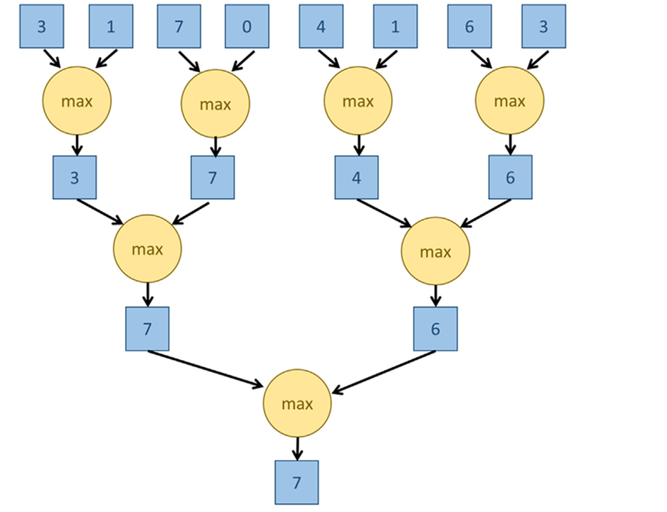
    Fig 26_01: Example illustratory diagram

  • This approach reduces computation time significantly compared to sequential methods.

Key Properties for Parallel Reduction: To perform parallel reduction effectively:

1. Associativity: The operator must be associative $(a \Theta b)\Theta c=a\Theta (b\Theta c)$. For example:
   • Addition and max are associative.
   • Subtraction is not.
2. Commutativity (optional): If $a\Theta b=b\Theta a$, we can rearrange operands freely for optimization.

Why Parallel Reduction is Faster:

In sequential reduction:

• Time steps = Number of elemnts $(N)$.

In parallel reduction:

• Time steps = $log_{2}(N)$.

For example:

• With $N = 8$, sequential reduction takes place 8 steps.
• Parallel reduction takes only $3$ steps !! ie.,$(log_{2}(8) = 3)$

However, parallel reduction requires more hardware resources initially (e.g., multiple comparators for max operations).

---

End of Day_26🫡