Summary of Day 21:

Starting Chapter 8: Stencil

Stencil Computation: What is it?

Stencil computations are a class of numerical algorithms used to update elements in a data grid based on neighboring values. They appear in many scientific and engineering applications, such as:

• Solving Partial Differential Equations (PDEs)
• Heat Diffusion Simulations
• Image Processing (Blurring, Edge Detection)
• Fluid Dynamics & Weather Simulation

Each point in a grid is updated by applying a fixed pattern (stencil) over its neighborhood.

---

Difference Between Stencil Computation and Convolution:

Though both apply a kernel to a region of data, they differ in intent:

Features	Stencil Computation	Convolution
Purpose	Used in PDEs, scientific computing	Mostly used in deep learning & signal/image processing
Operation	Updates each grid point based on its neighbors	Computes weighted sum using a kernel
Data Dependency	Strong dependencies on neighboring values	Often applied with independent operations

Stencil computations typically involve solving differential equations, while convolution is a mathematical operation used in filtering and feature extraction.

---

Stencils:

Definition: A stencil is a pattern of weights applied to grid points for numerical approximations of derivatives.

1. Finite-Difference Approximation For a function $f(x)$, the first derivative is approximated as:

f'(x) = \frac{f(x+h)- f(x-h)}{2h} + O(h^2)

where:

• $h$: grid spacing
• $O(h^2)$: error term, proportional to $h^2$

Discrete Derivative Example: Given grid array $F[i]$,

F_{D}[i] = \frac{F[i+1]- F[i-1]}{2h}

Rewriting as a weighted sum:

F_{D}[i] = - \frac{1}{2h}F[i-1] + \frac{1}{2h} F[i+1]

This defines a three-point stencil.

*Slight Notes:
Higher-Order Stencils

• Five-point stencil (second derivatives) involves $[i-2, i-1, i, i+1, i+2]$.
• Seven-point stencil (third derivatives) involves three points on either side and so on.

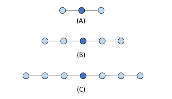
Fig 21_01: One-dimensional stencil examples. (A)Three-point (order1) stencil. (B)Five-point (order2) stencil. (C)Seven-point (order3) stencil.

2D Stencils

For PDEs with two variables $(x,y)$:

• Five-point stencil (Order 1): Uses grid points along x/y axes.
• Nine-point stencil (Order 2): Includes diagonals.

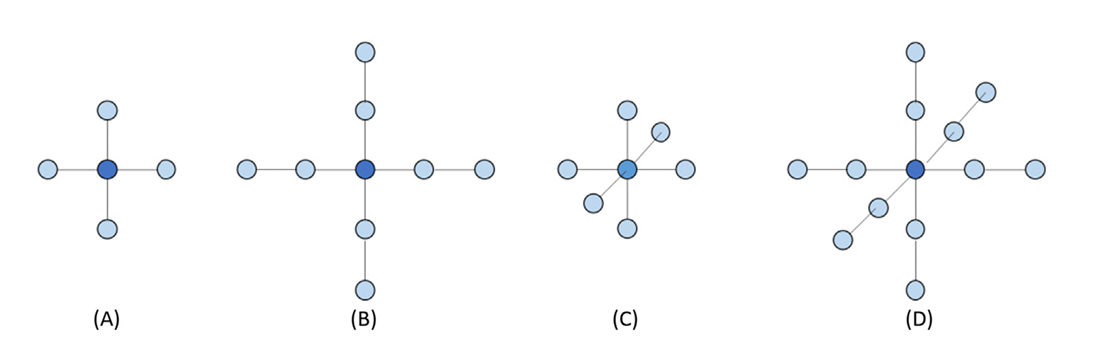
Fig 21_02: (A)Two-dimensional five-point stencil (order1).(B)Two-dimensional nine-point stencil (order2). (C)Three-dimensional seven-point stencil (order1). (D)Three-dimensional 13 point stencil (order2).

Parallel Stencil: A Basic Algorithm

Boundary Conditions: Boundary cells store fixed values and do not update during computation.

Kernel Code for basic CUDA for Stencil Swap:

__global__ void stencil_kernel(float* in, float* out, unsigned int N) {
    unsigned int i = blockIdx.z * blockDim.z + threadIdx.z;
    unsigned int j = blockIdx.y * blockDim.y + threadIdx.y;
    unsigned int k = blockIdx.x * blockDim.x + threadIdx.x;

    if (i >= 1 && i < N - 1 && j >= 1 && j < N - 1 && k >= 1 && k < N - 1) {
        out[i*N*N + j*N + k] = 
              c0 * in[i*N*N + j*N + k]
            + c1 * in[i*N*N + j*N + k - 1]
            + c2 * in[i*N*N + j*N + k + 1]
            + c3 * in[i*N*N + (j - 1)*N + k]
            + c4 * in[i*N*N + (j + 1)*N + k]
            + c5 * in[(i - 1)*N*N + j*N + k]
            + c6 * in[(i + 1)*N*N + j*N + k];
    }
}

The full code implementation: Click Here to redirect!

Performance Analysis: Each thread:

• Performs 13 floating-point operations (7 multiplications + 6 additions).
• Loads 7 input values from global memory.

Arithmetic Intensity:

  \text{Ratio} =  \frac{13}{7 \times 4} = 0.46 \space \text{OP/B}

This low ratio suggests the kernel is memory-bound.

Shared Memory Tiling for Stencil Sweep

Shared Memory Optimization:

Shared memory tiling reduces global memory access by caching reusable data on-chip.
Input tile: Includes halo regions around the output tile.

Kernel Code for Optimized Kernel using Shared Memory

__global__ void tiled_stencil_kernel(float* in, float* out, unsigned int N) {
    __shared__ float tile[IN_TILE_DIM][IN_TILE_DIM][IN_TILE_DIM];

    int i = blockIdx.z * OUT_TILE_DIM + threadIdx.z - HALO;
    int j = blockIdx.y * OUT_TILE_DIM + threadIdx.y - HALO;
    int k = blockIdx.x * OUT_TILE_DIM + threadIdx.x - HALO;

    if (i >= 0 && i < N && j >= 0 && j < N && k >= 0 && k < N) {
        tile[threadIdx.z][threadIdx.y][threadIdx.x] = in[i*N*N + j*N + k];
    }
    __syncthreads();

    if (threadIdx.z >= HALO && threadIdx.z < IN_TILE_DIM-HALO &&
        threadIdx.y >= HALO && threadIdx.y < IN_TILE_DIM-HALO &&
        threadIdx.x >= HALO && threadIdx.x < IN_TILE_DIM-HALO) {
        out[i*N*N + j*N + k] = 
              c0 * tile[threadIdx.z][threadIdx.y][threadIdx.x]
            + c1 * tile[threadIdx.z][threadIdx.y][threadIdx.x - 1]
            + c2 * tile[threadIdx.z][threadIdx.y][threadIdx.x + 1]
            + c3 * tile[threadIdx.z][threadIdx.y - 1][threadIdx.x]
            + c4 * tile[threadIdx.z][threadIdx.y + 1][threadIdx.x]
            + c5 * tile[threadIdx.z - 1][threadIdx.y][threadIdx.x]
            + c6 * tile[threadIdx.z + 1][threadIdx.y][threadIdx.x];
    }
}

Full code implementation: Click Here to redirect!

Key Optimizations:

• Shared memory stores input tiles to minimize global memory accesses.
• Threads load data collaboratively.
• Halo regions ensure boundary conditions.
• Synchronization (__syncthreads()) prevents race conditions.

Improved Arithmetic-to-Memory Ratio

With shared memory tiling:

\text{Ratio} = \frac{13(T-2)^3}{4T^3}

For large tiles $(T » Halo)$:

\text{Ratio} \approx 3.25 \space \text{OP/B}

Challenges with Small Tile Sizes:

• Small tiles (e.g., $T=8$) limit reuse ratio to $≈1.37 \space OP/B$.
• High halo overhead reduces efficiency.

---

End of Day_21🫡